Note

This tutorial was generated from a Jupyter notebook that can be downloaded here.

Ensemble analyses

In this tutorial we’ll show how to perform a very simple ensemble analysis to infer the statistical properties of the spots on a group of stars.

Generate the ensemble

In this section we will generate a synthetic ensemble of light curves of stars with “similar” spot properties. Let’s define some true values for the spot properties of the ensemble:

truths = {"r": 15, "mu": 30, "sigma": 5, "c": 0.05, "n": 20}

parameter	description	true value
r	mean radius in degrees	15
mu	latitude distribution mode in degrees	30
sigma	latitude distribution standard deviation in degrees	5
c	fractional spot contrast	0.05
n	number of spots	20

Now let’s generate 500 light curves from stars at random inclinations with spots drawn from the distributions above. We’ll do this by adding discrete circular spots to each star via the starry_process.calibrate.generate function. Note that in order to mimic real observations, we’ll normalize each light curve to its mean value and subtract unity to get the “relative” flux. For simplicity, we’ll give all of the light curves the same period and photometric uncertainty.

Note

The starry_process.calibrate module is used internally to verify the calibration of the Gaussian process, so it’s not very well documented. You can check out the list of valid keyword arguments to the generate function in this file.

from starry_process import calibrate

data = calibrate.generate(
    generate=dict(
        normalized=True,
        nlc=500,
        period=1.0,
        ferr=1e-3,
        nspots=dict(mu=truths["n"]),
        radius=dict(mu=truths["r"]),
        latitude=dict(mu=truths["mu"], sigma=truths["sigma"]),
        contrast=dict(mu=truths["c"]),
    )
)

100%|██████████| 500/500 [02:28<00:00,  3.37it/s]
100%|██████████| 500/500 [00:00<00:00, 17546.89it/s]

The variable data is a dictionary containing the light curves, the stellar maps (expressed as vectors of spherical harmonic coefficients y), plus some metadata.

t = data["t"]
flux = data["flux"]
ferr = data["ferr"]
y = data["y"]

Let’s visualize some of the light curves, all on the same scale:

import matplotlib.pyplot as plt

fig, ax = plt.subplots(3, 5)
for j, axis in enumerate(ax.flatten()):
    axis.plot(t, flux[j] * 1000)
    axis.set_ylim(-50, 50)
    axis.set_xticks([0, 1, 2, 3, 4])
    if j != 10:
        axis.set_xticklabels([])
        axis.set_yticklabels([])
    else:
        axis.set_xlabel("rotations")
        axis.set_ylabel("flux [ppt]");

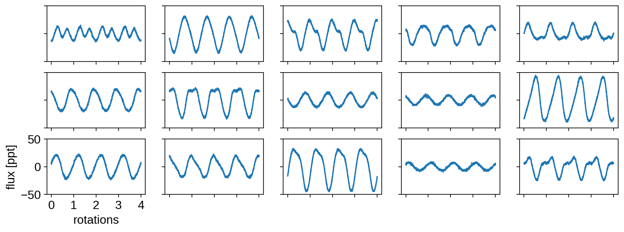
In the next section, we’ll assume we observe only these 500 light curves. We do not know the inclinations of any of the stars or anything about their spot properties: only that all the stars have statistically similar spot distributions.

Inference

Setup

Let’s set up a simple probabilistic model using pymc3 and solve for the five quantities above: the spot radius, the mode and standard deviation of the spot latitude, the spot contrast, and the number of spots. We’ll place uniform priors on everything except for the latitude mode mu, on which we’ll place an isotropic prior.

from starry_process import StarryProcess
import pymc3 as pm
import theano.tensor as tt
import numpy as np


with pm.Model() as model:

    # For use later
    varnames = ["r", "mu", "sigma", "c", "n"]

    # Spot latitude params. Isotropic prior on the mode
    # and uniform prior on the standard deviation
    u = pm.Uniform("u", 0, 1)
    mu = 90 - tt.arccos(u) * 180 / np.pi
    pm.Deterministic("mu", mu)
    sigma = pm.Uniform("sigma", 1.0, 20.0)

    # Spot radius (uniform prior)
    r = pm.Uniform("r", 10.0, 30.0)

    # Spot contrast & number of spots (uniform prior)
    c = pm.Uniform("c", 0.0, 0.5, testval=0.1)
    n = pm.Uniform("n", 1.0, 30.0, testval=5)

    # Instantiate the GP
    sp = StarryProcess(r=r, mu=mu, sigma=sigma, c=c, n=n)

    # Compute the log likelihood
    lnlike = sp.log_likelihood(t, flux, ferr ** 2, p=1.0)
    pm.Potential("lnlike", lnlike)

Note

Note that we explicitly provide a small testval for both the spot contrast and the number of spots. Otherwise, the initial value assumed in the optimization for both those quantities is the midpoint of the bounds (c = 0.5 and n = 25.5). That corresponds to a lot of very dark spots, which results in very high variance in the flux – too high, in fact, for the normalized Gaussian process to model! We discusss this in more detail in the paper. To avoid initializing the sampler in a bad region of parameter space, we provide a starting point that is guaranteed to lead to a finite log likelihood value.

Now that we’ve declared our model, we could go on to sample it using pymc3, e.g.,

with model:
    trace = pm.sample(
        tune=1000,
        draws=2000,
        cores=2,
        chains=2,
        init="adapt_full",
        target_accept=0.9,
    )

But in practice, it can be very difficult for the default Hamiltonian Monte Carlo algorithm to sample the posterior in these kinds of problems. There is probably some intelligent way to reparametrize the problem to make HMC sample the posterior efficiently, but we haven’t yet found it! Running the pymc3 sampler above generally takes a really long time\(-\)it can take minutes to draw a single sample!

We suspect that this is because the curvature of the posterior can be extremely variable, so methods that rely on first derivatives of the log probability (like HMC) struggle a lot. We’ve obtained far better performance using samplers that don’t rely on gradient evaluations (which are rather slow to compute anyways). In our paper, we used Nested Sampling (implemented in the dynesty package), but here we’ll use plain vanilla Markov Chain Monte Carlo (MCMC) as implemented in the emcee package.

To use emcee, we need a function that returns the log probability at a point. We could compile this ourselves from the log_likelihood method of our StarryProcess instance (plus a log prior term) using theano, but starry_process actually implements a simple MCMC interface to do this for us.

Let’s instantiate this interface, which automatically compiles the pymc3 model we defined above:

from starry_process import MCMCInterface

with model:
    mci = MCMCInterface()

Optimization

The first thing we can do with this interface object is to optimize the log probability function. This will get us the MAP (maximum a posteriori) solution, which is usually a good starting point for MCMC. Since we have so many light curves in our ensemble, it is actually also a good point estimate of the spot parameters.

x = mci.optimize()

optimizing logp for variables: [n, c, r, sigma, u]

100.00% [108/108 01:19<00:00 logp = 2.725e+06]

message: Desired error not necessarily achieved due to precision loss.
logp: 2724328.587834473 -> 2725135.770896861

The optimize method wraps a method with the same name in the pymc3_ext package (which in turn wraps scipy.optimize.minimize), so check those out for accepted keywords.

The optimization should have run in about a minute, which is fairly fast thanks to the availability of the gradient. (Even though HMC struggles, the gradient is still useful for optimization!)

Let’s check out the solution vector:

print(x)

[-0.52887785 -1.98579128 -0.93454528 -1.39502117 -0.00228807]

If these numbers don’t look right to you, it’s because they do not correspond to our spot parameters r, mu, sigma, etc. Instead, they are quantities in the parametrization used internally in pymc3, which maps our priors onto a space with infinite support. This makes it easy to sample over them, since we don’t need to specify hard bounds for any of them (they can take on any finite real value).

We’re going to run our sampler in this transformed space (in which our log probability function is defined) and transform back at the end. But we can take a peek at what they actually correspond to right now to check that our optimization worked correctly:

varnames = ["r", "mu", "sigma", "c", "n"]
mci.transform(x, varnames=varnames)

array([15.64006971, 29.96216293,  4.77353996,  0.06035142, 11.75258081])

Let’s compare these values to the true values:

parameter	description	true value	MAP value
r	mean radius in degrees	15	15.64
mu	latitude distribution mode in degrees	30	29.96
sigma	latitude distribution standard deviation in degrees	5	4.77
c	fractional spot contrast	0.05	0.0604
n	number of spots	20	11.75

Not bad! It seems that we correctly inferred all the properties (except for, maybe, the total number of spots; this quantity is generally not an observable in single-band photometry!)

But we don’t have any sense of the uncertainties on these quantities. For that, we need to run MCMC.

Posterior sampling

The first thing to do is define the initial point for each of the MCMC walkers (we’ll use 30). We can call the get_initial_state method to draw samples close to the MAP solution we obtained in the previous step. Note that this makes use of the estimate of the inverse Hessian matrix (returned by the optimizer), which can be somewhat numerically unstable. If this doesn’t work, try specifying a small variance var instead.

nwalkers = 30
p0 = mci.get_initial_state(nwalkers)

We’re now ready to run MCMC. We’ll instantiate a sampler and pass in mci.logp as our log probability\(-\)this is the automatically compiled function mentioned above. Since this notebook is running on GitHub Actions, we’ll run the chains for a measly 500 steps (although you should run it for much longer if you can!)

import emcee

# Number of parameters
ndim = p0.shape[1]

# Instantiate the sampler
sampler = emcee.EnsembleSampler(nwalkers, ndim, mci.logp)

# Run the chains
np.random.seed(0)
nsteps = 500
_ = sampler.run_mcmc(p0, nsteps, progress=True)

100%|██████████| 500/500 [31:54<00:00,  3.83s/it]

Let’s look at our chains, recalling that everything is still in the internal parametrization:

# Plot the walkers
fig, ax = plt.subplots(ndim, figsize=(8, 8), sharex=True)
for j in range(ndim):
    for k in range(nwalkers):
        ax[j].plot(sampler.chain[k, :, j], "C0-", lw=1, alpha=0.3)
    ax[j].set_ylabel("param {}".format(j + 1))
ax[-1].set_xlabel("iteration")
fig.align_ylabels(ax)
plt.show()

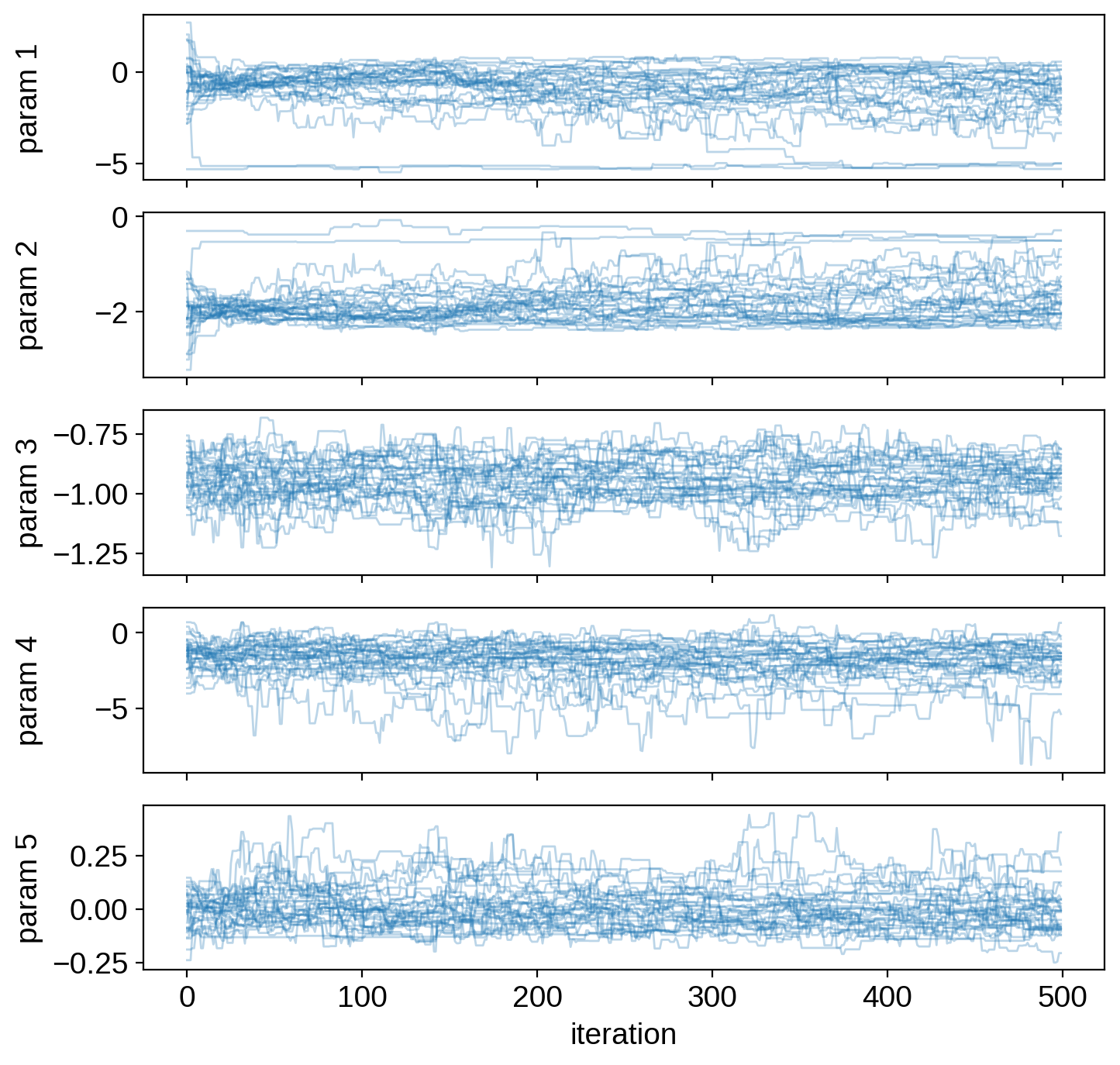
Note

Remember that we only ran these chains for 500 steps since we’re doing this on GitHub Actions. They’re definitely not converged! When you’re analyzing real data, make sure to run the chains for much longer.

Let’s get rid of the first 100 samples as burn-in and flatten everything into an array of shape (nsamples, ndim):

burnin = 100
samples = sampler.chain[:, burnin:, :].reshape(-1, ndim)

Next, let’s transform to our desired parametrization using the transform method:

samples = mci.transform(samples, varnames=varnames)

Finally, we can view the posteriors:

from corner import corner

corner(
    samples,
    labels=varnames,
    truths=[truths[name] for name in varnames],
    range=((10, 30), (0, 90), (1, 20), (0, 0.5), (1, 30)),
    truth_color="C1",
    bins=100,
    smooth=2,
    smooth1d=2,
)
plt.show()

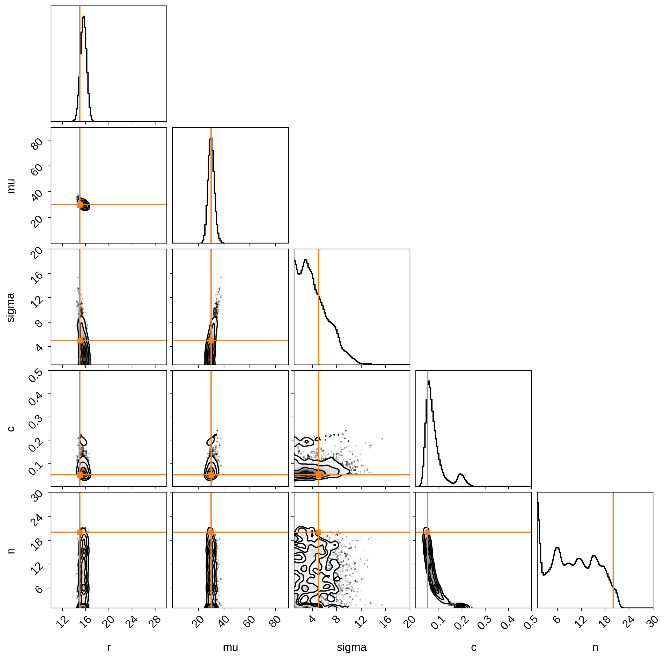
Not bad! Again, we seem to have correctly inferred everything except the number of spots, which is very unconstrained.