Note

This tutorial was generated from a Jupyter notebook that can be downloaded here.

Inference on time-variable stars

In this tutorial we’ll show how to infer spot properties from a star whose spots evolve in time. Check out the ensemble tutorial for a bit more information on how we’re doing our analysis here.

Generate

Let’s generate a synthetic light curve of a star with the following properties:

truths = dict(
    r=15.0,
    mu=30.0,
    sigma=5.0,
    c=0.05,
    n=20,
    tau=3.0,
    p=1.123,
    i=65.0,
    u=[0.0, 0.0],
    ferr=1e-3,
)
npts = 1500
tmax = 300.0

# Things we're solving for
varnames = ["r", "mu", "sigma", "c", "n", "i", "p", "tau"]

parameter	description	true value
r	mean radius in degrees	15.0
mu	latitude distribution mode in degrees	30.0
sigma	latitude distribution standard deviation in degrees	5.0
c	fractional spot contrast	0.05
n	number of spots	20
i	stellar inclination in degrees	65.0
p	stellar rotation period in days	1.123
tau	spot evolution timescale in days	3.0
u	limb darkening coefficients	[0.0, 0.0]
ferr	photometric uncertainty (fractional)	0.001
npts	number of points in light curve	1500
tmax	length of light curve in days	300.0

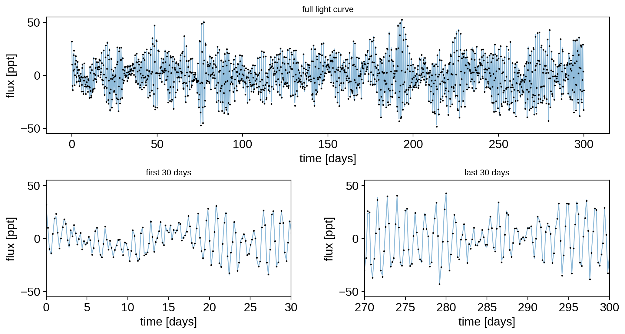
We will generate the light curve using a time-variable StarryProcess. If we were being rigorous about this, we should generate it from an actual forward model of a time-variable stellar surface. But that’s beyond the scope of this simple tutorial. Our goal here is to show that the light curve of a single star can encode most of the information we’re interested in if we observe it over many spot evolution timescales. This is something that cannot be done for a star with a static surface! The time variability is actually giving us lots of information about the covariance in the modes we’re able to probe at the particular inclination we see the star at.

from starry_process import StarryProcess
import numpy as np

t = np.linspace(0, tmax, npts)
sp = StarryProcess(**truths, marginalize_over_inclination=False)
flux0 = sp.sample(t, p=truths["p"], i=truths["i"], u=truths["u"]).eval()
flux = flux0 + truths["ferr"] * np.random.randn(*flux0.shape)

Here’s what our light curve looks like over all 300 days, as well as over the first and last 30 day segments:

import matplotlib.pyplot as plt


fig = plt.figure(figsize=(12, 6))
fig.subplots_adjust(hspace=0.4, wspace=0.3)
ax = [
    plt.subplot2grid((2, 2), (0, 0), colspan=2),
    plt.subplot2grid((2, 2), (1, 0)),
    plt.subplot2grid((2, 2), (1, 1)),
]
for axis in ax:
    axis.plot(t, 1e3 * flux0[0], "C0-", lw=1, alpha=0.5)
    axis.plot(t, 1e3 * flux[0], "k.", ms=2)
    axis.set_ylabel("flux [ppt]")
    axis.set_xlabel("time [days]")
    axis.set_ylim(-55, 55)
ax[0].set_title("full light curve", fontsize=10)
ax[1].set_title("first 30 days", fontsize=10)
ax[2].set_title("last 30 days", fontsize=10)
ax[1].set_xlim(0, 30)
ax[2].set_xlim(270, 300)
plt.show()

Inference

Let’s set up a simple probabilistic model using pymc3 to infer the spot properties of this star. We’ll place uninformative priors on everything, including the period, timescale, and inclination. For simplicity, let’s assume we know the limb darkening coefficients (which are zero in this case).

Note

Note that we are passing marginalize_over_inclination=False when instatiating our StarryProcess. That’s because we want to actually fit for the inclination of this star. Marginalizing over the inclination is useful when we’re analyzing a large ensemble of stars and don’t want to model the inclinations of every single one of them (which usually makes sampling trickier and slower).

import pymc3 as pm
import theano.tensor as tt


with pm.Model() as model:

    # Things we know
    u = truths["u"]
    ferr = truths["ferr"]

    # Spot latitude params. Isotropic prior on the mode
    # and uniform prior on the standard deviation
    unif0 = pm.Uniform("unif0", 0.0, 1.0)
    mu = 90 - tt.arccos(unif0) * 180 / np.pi
    pm.Deterministic("mu", mu)
    sigma = pm.Uniform("sigma", 1.0, 20.0)

    # Spot radius (uniform prior)
    r = pm.Uniform("r", 10.0, 30.0)

    # Spot contrast & number of spots (uniform prior)
    c = pm.Uniform("c", 0.0, 0.5, testval=0.1)
    n = pm.Uniform("n", 1.0, 30.0, testval=5)

    # Inclination (isotropic prior)
    unif1 = pm.Uniform("unif1", 0.0, 1.0)
    i = tt.arccos(unif1) * 180 / np.pi
    pm.Deterministic("i", i)

    # Period (uniform prior)
    p = pm.Uniform("p", 0.75, 1.25)

    # Variability timescale (uniform prior)
    tau = pm.Uniform("tau", 0.1, 10.0)

    # Instantiate the GP
    sp = StarryProcess(
        r=r, mu=mu, sigma=sigma, c=c, n=n, tau=tau, marginalize_over_inclination=False
    )

    # Compute the log likelihood
    lnlike = sp.log_likelihood(t, flux, ferr ** 2, p=p, i=i, u=u)
    pm.Potential("lnlike", lnlike)

As we discussed in this tutorial, it can be very difficult to sample the posterior for a StarryProcess problem using Hamiltonian Monte Carlo. It’s often much easier to use regular old-fashioned MCMC, which we can easily due via the MCMCInterface class:

from starry_process import MCMCInterface

with model:
    mci = MCMCInterface()

Let’s run the optimizer to find the maximum a posteriori (MAP) solution:

x = mci.optimize()

optimizing logp for variables: [tau, p, unif1, n, c, r, sigma, unif0]

100.00% [143/143 02:17<00:00 logp = 5.456e+03]

message: Desired error not necessarily achieved due to precision loss.
logp: 2020.3826546101209 -> 5455.770611578508

Recall that we need to transform the solution from the internal parametrization to our desired parametrization (in terms of the spot radius, spot latitude, etc.):

map_soln = mci.transform(x, varnames=varnames)

parameter	description	true value	MAP value
r	mean radius in degrees	15.0	14.17
mu	latitude distribution mode in degrees	30.0	26.77
sigma	latitude distribution standard deviation in degrees	5.0	9.28
c	fractional spot contrast	0.05	0.0730
n	number of spots	20	11.92
i	stellar inclination in degrees	65.0	63.90
p	stellar rotation period in days	1.123	1.13
tau	spot evolution timescale in days	3.0	2.98

Not bad! It looks like we correctly estimated several of the properties of interest! We still don’t have any sense of the uncertainty on these quantities; for that, we need to actually run the MCMC sampler.

nwalkers = 30
p0 = mci.get_initial_state(nwalkers)

Note

Since we’re running this example on GitHub Actions, we’ll only run the chain for 1000 steps, so it won’t be converged. You should run it for much, much longer if you can!

import emcee

# Number of parameters
ndim = p0.shape[1]

# Instantiate the sampler
sampler = emcee.EnsembleSampler(nwalkers, ndim, mci.logp)

# Run the chains
np.random.seed(0)
nsteps = 1000
_ = sampler.run_mcmc(p0, nsteps, progress=True)

100%|██████████| 1000/1000 [1:33:43<00:00,  5.62s/it]

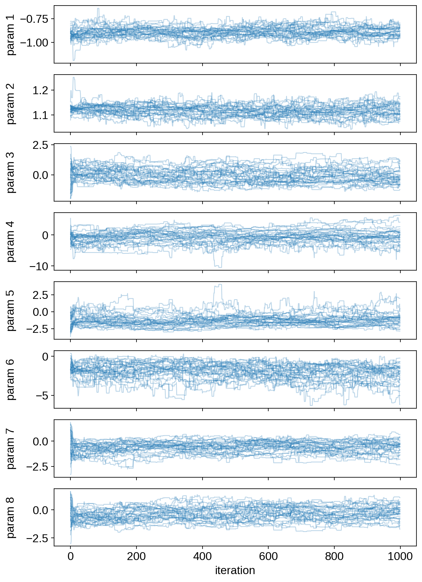
Let’s plot the chains:

# Plot the walkers
fig, ax = plt.subplots(ndim, figsize=(8, 12), sharex=True)
for j in range(ndim):
    for k in range(nwalkers):
        ax[j].plot(sampler.chain[k, :, j], "C0-", lw=1, alpha=0.3)
    ax[j].set_ylabel("param {}".format(j + 1))
ax[-1].set_xlabel("iteration")
fig.align_ylabels(ax)
plt.show()

Remove some burn-in and flatten the samples:

burnin = 200
samples = sampler.chain[:, burnin:, :].reshape(-1, ndim)

Transform to our parametrization:

samples = mci.transform(samples, varnames=varnames)

Visualize the posteriors, with the true values in orange:

from corner import corner

corner(
    samples,
    labels=varnames,
    truths=[truths[name] for name in varnames],
    range=(
        (10, 30),
        (0, 90),
        (1, 20),
        (0, 0.5),
        (1, 30),
        (0, 90),
        (0.75, 1.25),
        (0.1, 10.0),
    ),
    truth_color="C1",
    bins=100,
    smooth=2,
    smooth1d=2,
)
plt.show()

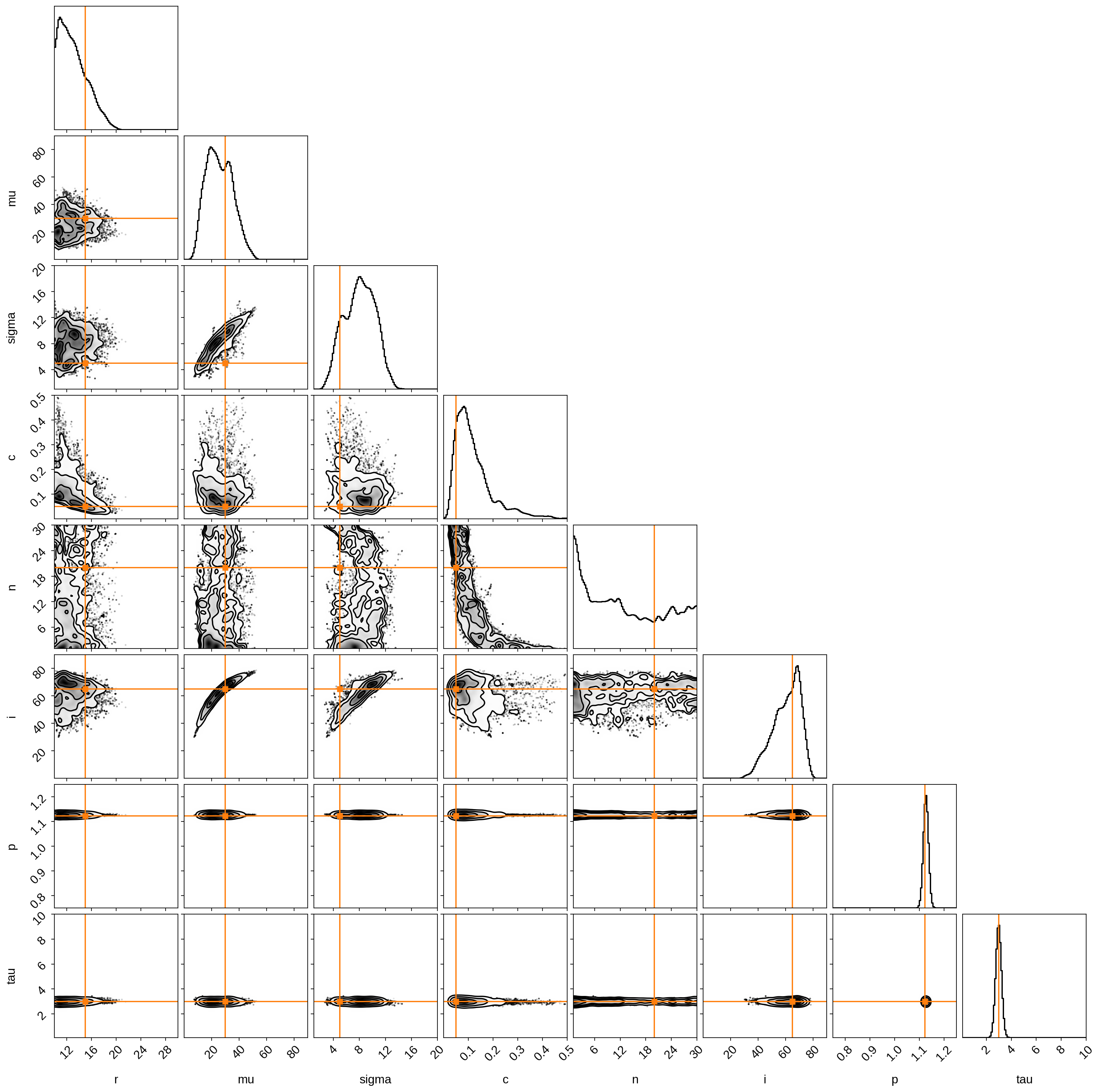
We did pretty good! Time-variable light curves encode a lot of the information we need, provided we observe the star over many (i.e., hundreds!) evolution timescales.