Note

This tutorial was generated from a Jupyter notebook that can be downloaded here.

Inferring spot latitudes

In the Quickstart tutorial, we showed how to infer the radii of the star spots in a (very simple) example. In this notebook we’ll discuss how to infer the parameters controlling their distribution in latitude.

Setup

Let’s import some basic stuff. We’ll use the emcee package to run our MCMC analyses below.

from starry_process import StarryProcess, beta2gauss
import numpy as np
import matplotlib.pyplot as plt
from tqdm.auto import tqdm
import theano
import theano.tensor as tt
import emcee
from corner import corner

We’ll instantiate a StarryProcess with high-latitude spots at \(\phi = 60^\circ \pm 5^\circ\):

truths = [60.0, 5.0]
sp = StarryProcess(mu=truths[0], sigma=truths[1])

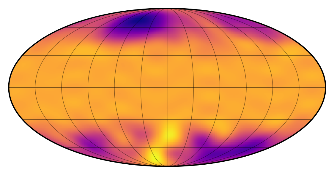
Here’s what a random sample from the process looks like on the surface of the star:

sp.visualize()

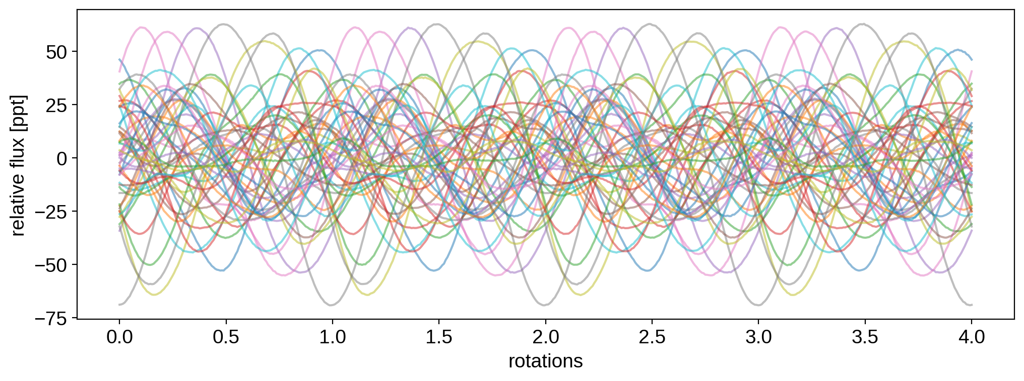
To start us off, let’s draw 50 light curve samples from the process:

t = np.linspace(0, 4, 500)
flux = sp.sample(t, nsamples=50).eval()
flux.shape

(50, 500)

All samples have the same rotation period (1.0 day by default), and we’re computing the light curves over 4 rotations. Since by default StarryProcess marginalizes over inclination, these samples correspond to random inclinations drawn from an isotropic distribution. Let’s visualize all of them:

for k in range(50):
    plt.plot(t, 1e3 * flux[k], alpha=0.5)
plt.xlabel("rotations")
plt.ylabel("relative flux [ppt]")
plt.show()

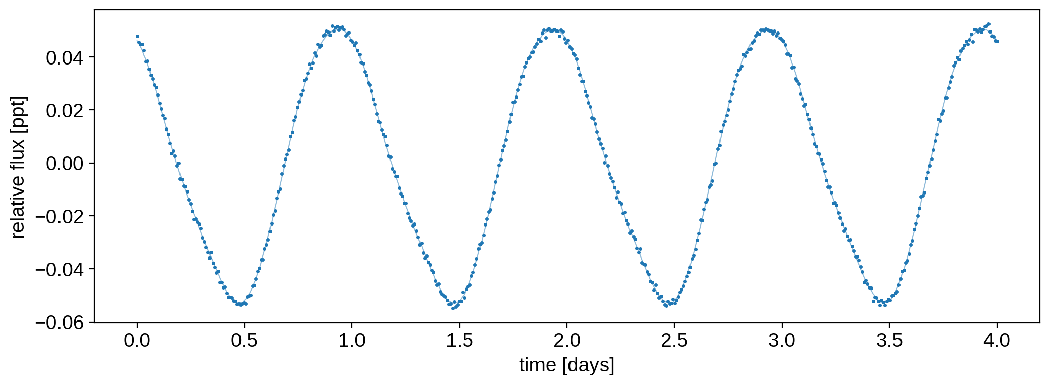
Since we’re going to do inference, we need to add a bit of observational noise to these samples to mimic actual observations. Here’s what the first light curve looks like:

ferr = 1e-3
np.random.seed(0)
f = flux + ferr * np.random.randn(50, len(t))
plt.plot(t, flux[0], "C0-", lw=0.75, alpha=0.5)
plt.plot(t, f[0], "C0.", ms=3)
plt.xlabel("time [days]")
plt.ylabel("relative flux [ppt]")
plt.show()

MCMC

Given these 50 light curves, our task now is to infer the mean and standard deviation of the spot latitude distribution. For simplicity, we’ll assume we know everything else: the spot radius, contrast, number of spots, and stellar rotation period (but not the inclinations). That makes the inference problem 2-dimensional and thus fast to run.

Note

In two dimensions, it’s usually more efficient to grid up the space, compute the likelihood everywhere on the grid, then sum it up to find the normalization constant directly and thus obtain the posterior. But since most use cases will be > 2d, we’ll do inference here using MCMC as an example.

A few notes about this. First, the spot latitude distribution assumed internally is not a Gaussian. It’s a Beta distribution in the cosine of the latitude, which in certain limits looks a lot like a bimodal Gaussian, with a mode at \(+\mu_\sigma\) and a mode at \(-\mu_\sigma\). The parameters of this distribution are the mode mu and the local standard deviation at the mode sigma, which in many cases are good approximations to the mean and standard deviation of the closest-matching Gaussian. The reason for this is explained in the paper: the adopted distribution and parametrization admits a closed-form solution to the mean and covariance of the GP, which is at the heart of why starry_process is so fast.

For reference, you can compute the actual distribution assumed internally by calling

sp.latitude.pdf(phi)

where sp is an instance of StarryProcess (with certain values of mu and sigma), and phi is the latitude(s) in degrees at which to compute the probability density function (PDF). Here’s the distribution we used to generate the light curve samples:

phi = np.linspace(-90, 90, 1000)
pdf = sp.latitude.pdf(phi).eval()
plt.plot(phi, pdf)
plt.xlabel("latitude [degrees]")
plt.ylabel("probability density")
plt.show()

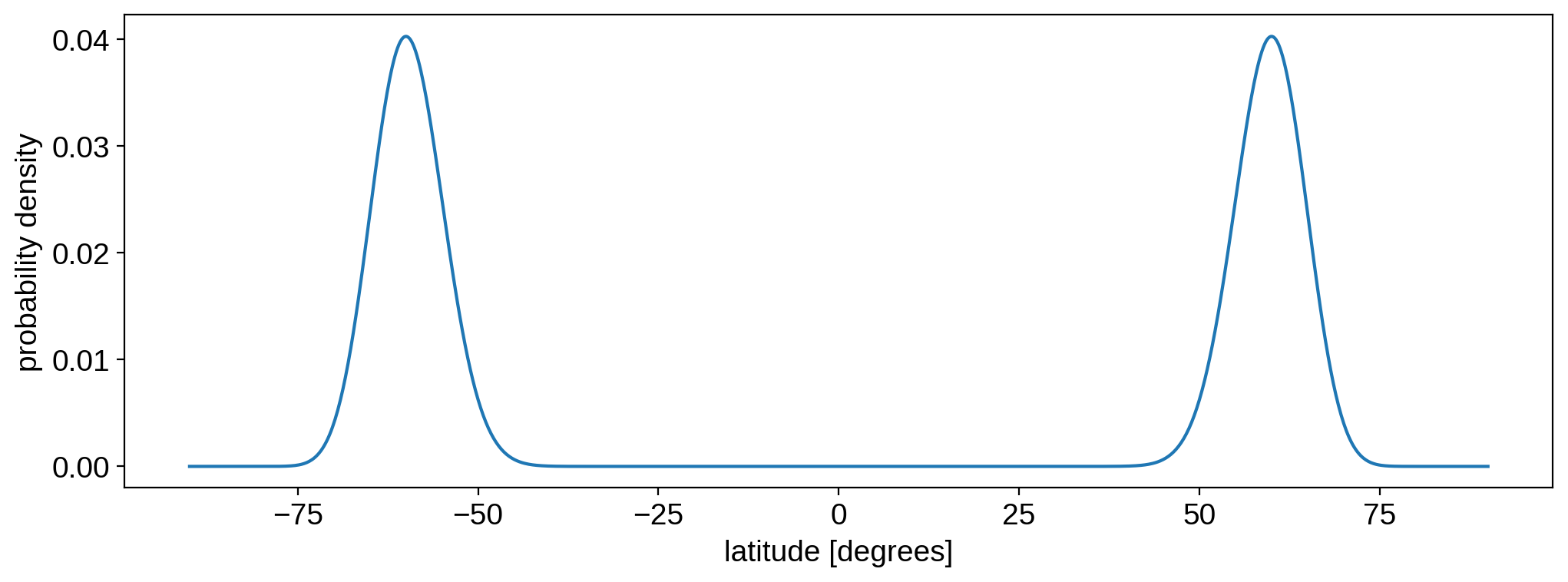
As promised, it looks a lot like a bimodal Gaussian with mean mu = 60 and standard deviation sigma = 5. Typically, this distribution deviates from a Gaussian when either mu or sigma get very large.

The other thing to note before we do inference is that there are two ways of proceeding. We can either sample in the parameters mu and sigma or in the dimensionless parameters a and b. In most cases we’ll get the same answer (provided we account for the Jacobian of the transformation), but we recommend the latter as it’s guaranteed to be numerically stable. That’s because there are certain combinations of mu and sigma that lead to very large coefficients in the evaluation of the integrals of the Beta distribution. This usually happens when sigma is very small (less than 1 or 2 degrees) or mu is very large (larger than 85 degrees). Sometimes this can raise errors in the likelihood evaluation (which can be caught in a try...except block), but sometimes it can just silently lead to the wrong value of the likelihood. The latter can be avoided by limiting the prior bounds on these two quantities. We do this below, and show that for this specific example, it works great!

However, a better approach is to sample in the dimensionless parameters a and b, which both have support in [0, 1], then transform the posterior constraints on these parameters into constraints on mu and sigma. Sampling in this space is much, much more likely to work seamlessly. We’ll discuss how to do this below. But first, let’s show how to sample in mu and sigma directly.

Sampling in mu, sigma

As in the Quickstart tutorial, we need to compile our likelihood function. We’ll make it a function of the scalars mu and sigma, and bake in the time array t, the batch of light curves f, and the photometric uncertainty ferr (as well as all the other default hyperparameter values).

mu_tensor = tt.dscalar()
sigma_tensor = tt.dscalar()
log_likelihood1 = theano.function(
    [mu_tensor, sigma_tensor],
    StarryProcess(mu=mu_tensor, sigma=sigma_tensor).log_likelihood(t, f, ferr ** 2),
)

Note

In some of the other tutorials, we compute the joint log likelihood of all the light curves in an ensemble by summing the log likelihood of each one. This requires as many function calls as there are light curves (50 in this case), which can lead to painfully slow runtimes. We can drastically improve on this by passing in all the light curves at once as a matrix whose rows are individual light curves, which will re-use the factorization of the covariance matrix for all of them. However, this assumes that all stars have the same hyperparameters, including the rotation period, limb darkening coefficients, and the photometric uncertainty (but not the inclination, since we’re marginalizing over it). In this particular example, all stars have the same period and photometric uncertainty (and no limb darkening), so we can get away with this shortcut. But in general, this will not be the correct approach!

We can now construct our log probability function (the sum of the log likelihood and the log prior). Let’s adopt the simplest possible prior: a uniform distribution for mu and sigma that avoids the unstable values discssued above. We’ll draw from this prior to obtain our initial sampling point, p0:

def log_prob1(x):
    mu, sigma = x
    if (mu < 0) or (mu > 85):
        return -np.inf
    elif (sigma < 1) or (sigma > 30):
        return -np.inf
    return log_likelihood1(mu, sigma)


ndim, nwalkers = 2, 6
p0 = np.transpose(
    [np.random.uniform(0, 85, size=nwalkers), np.random.uniform(1, 30, size=nwalkers)]
)

Now we can instantiate a sampler (using emcee) and run it. We’ll do 1000 steps with 6 walkers:

sampler1 = emcee.EnsembleSampler(nwalkers, ndim, log_prob1)
_ = sampler1.run_mcmc(p0, 1000, progress=True)
chain1 = np.array(sampler1.chain)

100%|██████████| 1000/1000 [05:13<00:00,  3.19it/s]

Here is the trace plot:

fig, ax = plt.subplots(2)
for k in range(nwalkers):
    ax[0].plot(chain1[k, :, 0])
    ax[1].plot(chain1[k, :, 1])
ax[0].set_ylabel(r"$\mu$ [deg]")
ax[1].set_ylabel(r"$\sigma$ [deg]")
ax[1].set_xlabel("iteration")
plt.show()

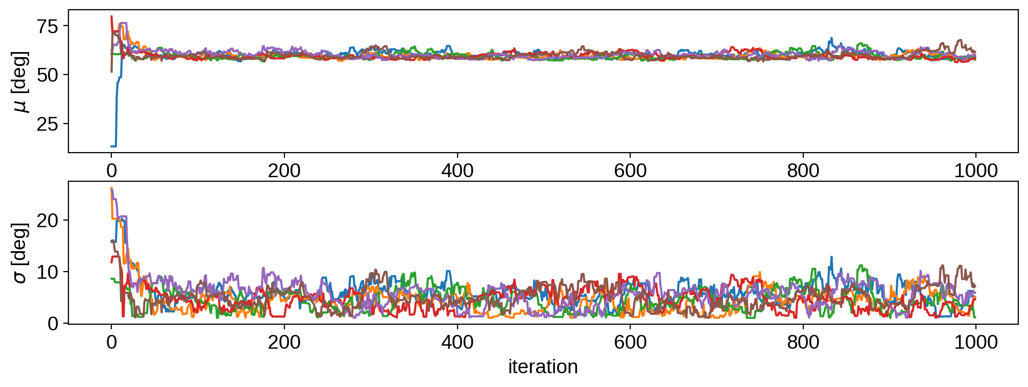
This has definitely not converged, but it’s good enough for our toy example. Let’s remove the first 100 samples as our burn-in and plot the joint posterior:

corner(chain1[:, 100:, :].reshape(-1, 2), truths=truths, labels=["$\mu$", "$\sigma$"])
plt.show()

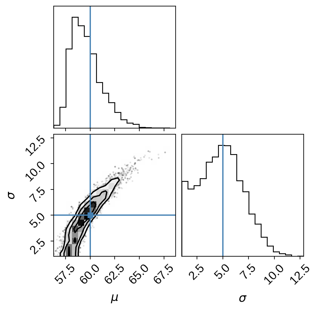
Not bad! The true values are indicated in blue. We correctly infer the presence of high-latitude spots! Note, however, the degeneracy here. It’s difficult to rule out polar spots with high variance! We discuss this at length in the paper. Pay attention to the curvature of the degeneracy, which gets worse for higher latitude spots. In some cases, this might be a very hard posterior to sample using MCMC!

Sampling in a, b

As we mentioned above, it’s preferable to sample in the dimensionless parameters a and b, which are just a (nonlinear) transformation of mu and sigma onto the unit square. There is a one-to-one correspondence between the two sets of quantities. Converting between them can be done via the utility functions

mu, sigma = starry_process.beta2gauss(a, b)

and

a, b = starry_process.gauss2beta(mu, sigma)

Let’s compile our likelihood function to take a and b as input:

a_tensor = tt.dscalar()
b_tensor = tt.dscalar()
sp = StarryProcess(a=a_tensor, b=b_tensor)
log_likelihood2 = theano.function(
    [a_tensor, b_tensor],
    sp.log_likelihood(t, f, ferr ** 2) + sp.log_jac(),
)

Note that we added an extra term in the computation of the likelihood: sp.log_jac(). This is the log of the absolute value of the determinant of the Jacobian of the transformation (ugh!), which corrects for the (very wonky) implicit prior introduced by our reparametrization. By adding this term, we can place a uniform prior on a and b in [0, 1] and effectively obtain a uniform prior on mu and sigma when we transform our posterior constraints below.

Here’s our log probability function, with the trivial prior on a and b:

def log_prob2(x):
    a, b = x
    if (a < 0) or (a > 1):
        return -np.inf
    elif (b < 0) or (b > 1):
        return -np.inf
    return log_likelihood2(a, b)


ndim, nwalkers = 2, 6
p0 = np.random.uniform(0, 1, size=(nwalkers, 2))

Let’s run the sampler as before:

sampler2 = emcee.EnsembleSampler(nwalkers, ndim, log_prob2)
_ = sampler2.run_mcmc(p0, 1000, progress=True)
chain2_ab = np.array(sampler2.chain)

100%|██████████| 1000/1000 [05:37<00:00,  2.97it/s]

Our samples are in the dimensionless quantities a and b, but what we really want are samples in mu and sigma. Let’s use the utility function mentioned above to transform them:

chain2 = np.zeros_like(chain2_ab)
for k in range(nwalkers):
    for n in range(1000):
        chain2[k, n] = beta2gauss(*chain2_ab[k, n])

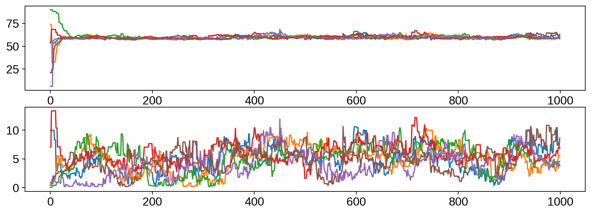
Here’s the trace plot:

fig, ax = plt.subplots(2)
for k in range(nwalkers):
    ax[0].plot(chain2[k, :, 0])
    ax[1].plot(chain2[k, :, 1])

and, finally, the joint posterior:

corner(chain2[:, 100:, :].reshape(-1, 2), truths=truths, labels=["$\mu$", "$\sigma$"])
plt.show()

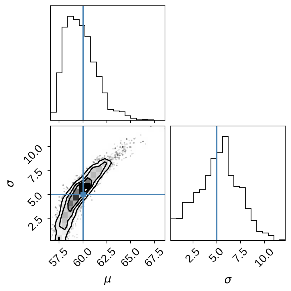
As expected, we get very similar results (keeping in mind the chains are still very far from convergence!)

Bottom line: you can sample in whichever parametrization you want, but we recommend using a and b as your parameters, as long as you remember to add the Jacobian term to the likelihood.

Note

If you’re explicitly summing log-likelihoods in an ensemble analysis, remember that you only want to add the log Jacobian a single time!