Note

This tutorial was generated from a Jupyter notebook that can be downloaded here.

Time variability

In this tutorial, we will cover how to instantiate a time-variable StarryProcess, useful for modeling stars with spots that evolve over time. We will show how to sample from the process and use it to do basic inference.

Setup

from starry_process import StarryProcess
import numpy as np
import matplotlib.pyplot as plt
from tqdm.auto import tqdm
import theano
import theano.tensor as tt

To instantiate a time-variable StarryProcess, we simply pass a nonzero value for the tau parameter:

sp = StarryProcess(tau=25.0)

This is the timescale of the surface evolution in arbitrary units (i.e., this will have the same units as the rotation period and the input time arrays; units of days are the common choice). We can also provide a GP kernel to model the time variability. By default a Matern-3/2 kernel is used, but that can be changed by supplying any of the kernels defined in the starry_process.temporal module with the kernel keyword. If you wish, you can even provide your own callable tensor-valued function of the form

def kernel(t1, t2, tau):
    (...)
    return K

where t1 and t2 are the input times (scalars or vectors), tau is the timescale, and K is a covariance matrix of shape (len(t1), len(t2)).

Let’s stick with the Matern32 kernel for now, and specify a time array over which we’ll evaluate the process:

t = np.linspace(0, 50, 1000)

Sampling

Sampling in spherical harmonics

The easiest thing we can do is sample maps. For time-variable processes, we can pass a time t argument to sample_ylm to get map samples evaluated at different points in time:

y = sp.sample_ylm(t).eval()
y

array([[[ 1.98197320e-06, -3.81494229e-03,  9.46731253e-03, ...,
         -1.61085768e-03, -1.21449760e-03,  2.61072812e-03],
        [ 1.98777316e-06, -3.72789607e-03,  9.40451471e-03, ...,
         -1.60980601e-03, -1.21834164e-03,  2.60772801e-03],
        [ 1.99385141e-06, -3.64801549e-03,  9.33341106e-03, ...,
         -1.60858574e-03, -1.22108089e-03,  2.60411143e-03],
        ...,
        [ 3.97931987e-07,  8.24640989e-03, -2.11995612e-02, ...,
          5.60005483e-04, -1.51144082e-03,  1.51503708e-03],
        [ 3.93531768e-07,  8.23100279e-03, -2.13551280e-02, ...,
          5.49545554e-04, -1.49624829e-03,  1.51438914e-03],
        [ 3.88700646e-07,  8.21886595e-03, -2.15127955e-02, ...,
          5.39429601e-04, -1.48113806e-03,  1.51377761e-03]]])

Note the shape of y, which is (number of samples, number of times, number of ylms):

y.shape

(1, 1000, 256)

At every point in time, the spherical harmonic representation of the surface is different. We can visualize this as a movie by simply calling

sp.visualize(y)

Computing the corresponding light curve is easy:

flux = sp.flux(y, t).eval()
flux

array([[-0.01631175, -0.01916606, -0.02341942, ...,  0.00161407,
        -0.01026314, -0.02248795]])

where the shape of flux is (number of samples, number of times):

flux.shape

(1, 1000)

We could also pass explicit values for the following parameters (otherwise they assume their default values):

attribute	description	default value
i	stellar inclination in degrees	60.0
p	stellar rotation period in days	1.0
u	limb darkening coefficient vector	[0. 0.]

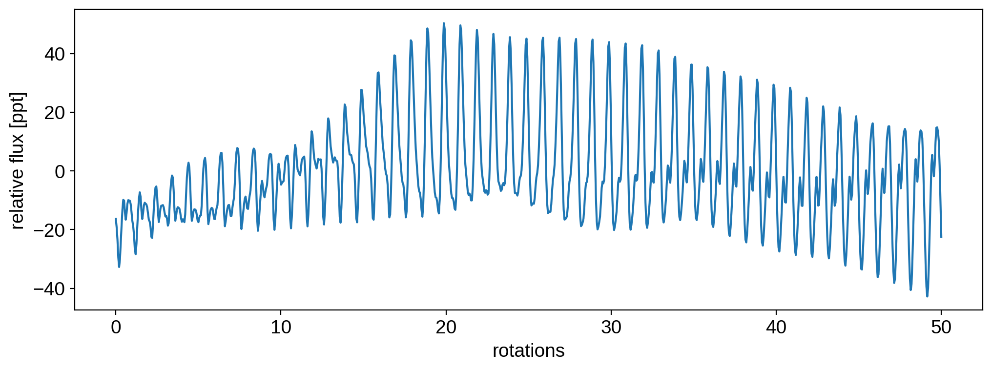
Here’s the light curve in parts per thousand:

plt.plot(t, 1e3 * flux[0])
plt.xlabel("rotations")
plt.ylabel("relative flux [ppt]")
plt.show()

Sampling in flux

We can also sample in flux directly:

flux = sp.sample(t, nsamples=50).eval()
flux

array([[ 0.07838618,  0.06464705,  0.04244707, ...,  0.06331804,
         0.05142009,  0.0365836 ],
       [ 0.01378447,  0.02370538,  0.03521725, ..., -0.04152575,
        -0.04475802, -0.04349481],
       [ 0.0590112 ,  0.06348585,  0.0546207 , ..., -0.02683003,
        -0.04158381, -0.04769547],
       ...,
       [-0.05463797, -0.07863731, -0.09790254, ...,  0.05184834,
         0.03765136,  0.01797497],
       [ 0.00605763,  0.0012725 , -0.00351335, ..., -0.04518317,
        -0.01887255,  0.00907892],
       [ 0.02490599,  0.0453551 ,  0.05680081, ...,  0.0147044 ,
         0.00834349,  0.0005404 ]])

where again it’s useful to note the shape of the returned quantity, (number of samples, number of time points):

flux.shape

(50, 1000)

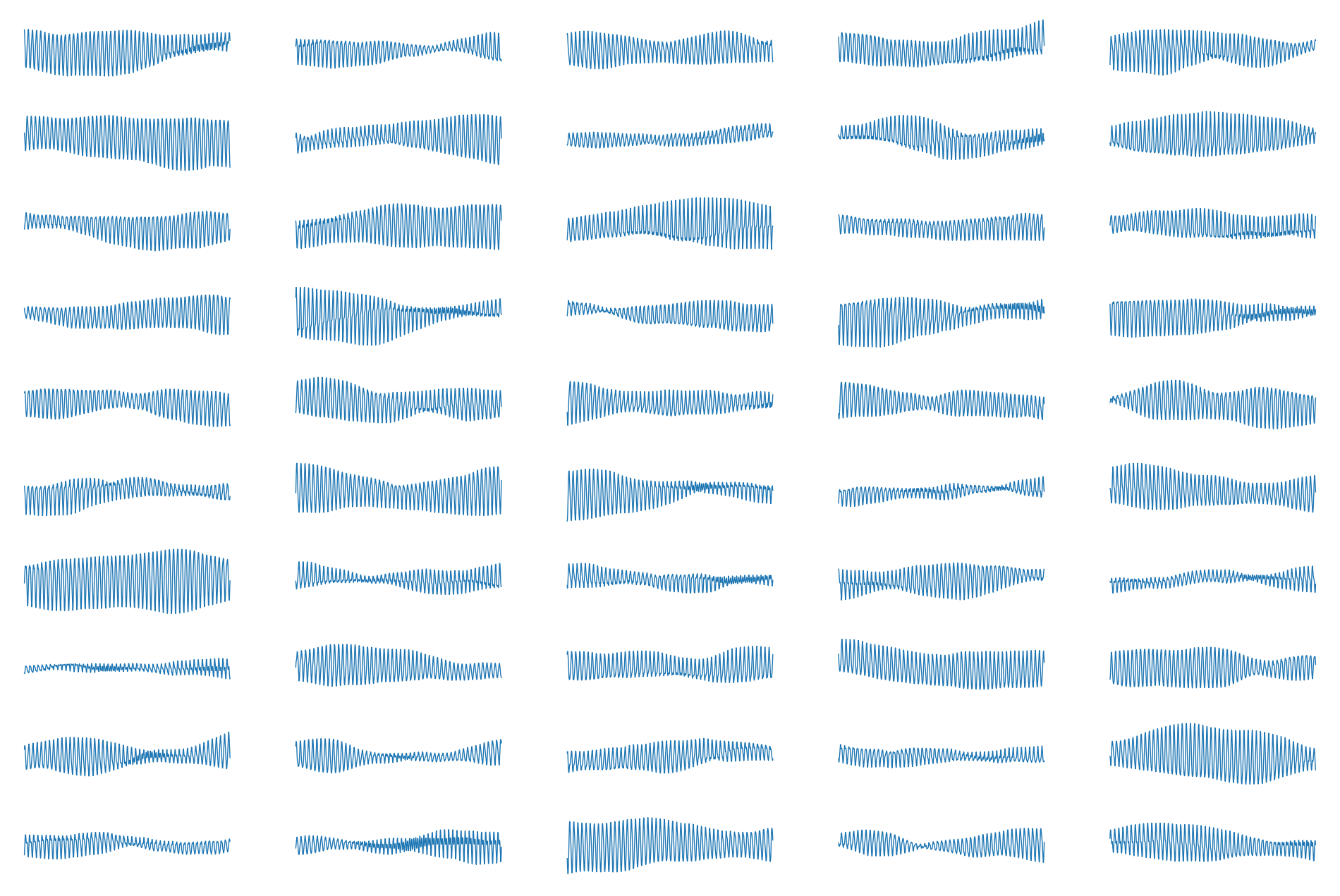
Here are all 50 light curves plotted on the same scale:

fig, ax = plt.subplots(10, 5, figsize=(12, 8), sharex=True, sharey=True)
ax = ax.flatten()
for k in range(50):
    ax[k].plot(t, 1e3 * flux[k], lw=0.5)
    ax[k].axis("off")

Doing inference

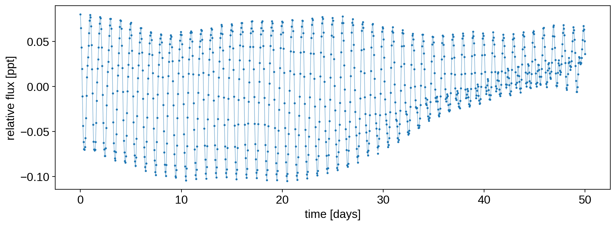
We can also do inference using time-variable StarryProcess models. Let’s do a mock ensemble analysis on the 50 light curves we generated above. First, let’s add some observation noise. Here’s what the first “observed” light curve looks like:

ferr = 1e-3
np.random.seed(0)
f = flux + ferr * np.random.randn(50, len(t))
plt.plot(t, flux[0], "C0-", lw=0.75, alpha=0.5)
plt.plot(t, f[0], "C0.", ms=3)
plt.xlabel("time [days]")
plt.ylabel("relative flux [ppt]")
plt.show()

Now, let’s try to infer the timescale of the generating process. For simplicity, we’ll keep all other parameters fixed at their default (and in this case, true) values. As in the Quickstart tutorial, we compile the likelihood function using theano. It will accept two inputs, a light curve and a timescale, and will return the corresponding log likelihood. To make this example run a little faster, we’ll also downsample the light curves by a factor of 5 (not recommended in practice! We should never throw out information!)

f_tensor = tt.dvector()
tau_tensor = tt.dscalar()
log_likelihood = theano.function(
    [f_tensor, tau_tensor],
    StarryProcess(tau=tau_tensor).log_likelihood(t[::5], f_tensor[::5], ferr ** 2),
)

Compute the joint likelihood of all datasets:

tau = np.linspace(0, 50, 100)
ll = np.zeros_like(tau)
for k in tqdm(range(len(tau))):
    ll[k] = np.sum([log_likelihood(f[n], tau[k]) for n in range(50)])

Following the same steps as in the Quickstart tutorial, we can convert this into a posterior distribution by normalizing it (and implicitly assuming a uniform prior over tau):

likelihood = np.exp(ll - np.max(ll))
prob = likelihood / np.trapz(likelihood, tau)
plt.plot(tau, prob, label="posterior")
plt.axvline(25, color="C1", label="truth")
plt.legend()
plt.ylabel("probability density")
plt.xlabel("variability timescale [days]")
plt.show()

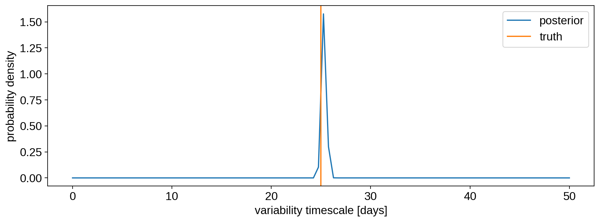
As expected, we correctly infer the timescale of variability.